I am fascinated by the beauty of music, which motivated me to play around with Digital Signal Processing. In order to better understand both music and DSP, I created a tool that can plot visually pleasing waveforms of audio files. The source code is available on GitHub as the Beautiful Sound project.

Below you can find the waveform of Heart’s Mystery Unfolding by Paul Baker. If you would like to see more images like this, you are more than welcome to visit Beautiful Sound’s homepage. The images look best in HD, so make sure to click and zoom in!


Our new paper, Hyperparameter Tuning in Bandit-Based Adaptive Operator Selection, was accepted to EvoApplications 2012. Here’s the abstract:

We are using bandit-based adaptive operator selection while autotuning parallel computer programs. The autotuning, which uses evolutionary algorithm-based stochastic sampling, takes place over an extended duration and occurs in situ as programs execute. The environment or context during tuning is either largely static in one scenario or dynamic in another. We rely upon adaptive operator selection to dynamically generate worthy test configurations of the program. In this paper, we study how the choice of hyperparameters, which control the trade-off between exploration and exploitation, affects the effectiveness of adaptive operator selection which in turn affects the performance of the autotuner. We show that while the optimal assignment of hyperparameters varies greatly between different benchmarks, there exists a single assignment, for a context, of hyperparameters that performs well regardless of the program being tuned.

I had a hard time finding a simple and easy-to-use library in Python that would let me draw on PNG images by directly manipulating pixel data. libcairo‘s ImageSurface works well, but the color component ordering is a bit unusual (BGRA) and coordinates have to be manually translated to an array index. You also have to worry about converting data back and forth between bytes (characters) and numeric types. Below you can find a thin wrapper that abstracts away those operations:

class PngImage:
    def __init__(self, surface):
        self.surface = surface;
        self.bpp = 4 # alpha ignored but still present in RGB24
        self.data = self.surface.get_data()    
 
    @classmethod
    def create(cls, w, h):
        return PngImage(ImageSurface(FORMAT_ARGB32, w, h))
 
    @classmethod
    def load(cls, file):
        return PngImage(ImageSurface.create_from_png(file))
 
    def write(self, file):
        self.surface.write_to_png(file)
 
    def height(self):
        return self.surface.get_height()
 
    def width(self):
        return self.surface.get_width()
 
    def coordinates_to_index(self, x, y):
        return self.bpp*(y*self.width() + x)
 
    def set_pixel(self, x, y, color, alpha=255):
        (r, g, b) = color
        i = self.coordinates_to_index(x,y)
        d = self.data
        d[i] = chr(b)
        d[i+1] = chr(g)
        d[i+2] = chr(r)
        if self.surface.get_format() == FORMAT_ARGB32:
            d[i+3] = chr(alpha)
 
    def get_pixel(self, x, y):
        i = self.coordinates_to_index(x,y)
        d = self.data
        return (ord(d[i+2]), ord(d[i+1]), ord(d[i]),
                ord(d[i+3]) if self.surface.get_format() == FORMAT_ARGB32
                            else None)

I hope the methods are self-explanatory. Here’s how PngImage could be used to add a ripple effect to a PNG file:

# returns a ripple magnitude in the range [0.5; 1]
def compute_z(x, y, x0, y0):
    r = sqrt((x-x0)**2 + (y-y0)**2)
    return (3.0 + cos(0.001*r*r))/4.0
 
if __name__ == "__main__":
    if(len(sys.argv) < 3):
        sys.stderr.write("usage: %s INPUT.PNG OUTPUT.PNG\n" % sys.argv[0])
        exit(1)
 
    src_img = PngImage.load(sys.argv[1])
    dest_img = PngImage.create(src_img.width(), src_img.height())
 
    # compute and write ripple pixels
    (x0,y0) = (src_img.width()/2, src_img.height()/2)
    for y in range(src_img.height()):
        for x in range(src_img.width()):
            (r, g, b, a) = src_img.get_pixel(x, y)
            z = compute_z(x, y, x0, y0)
            dest_img.set_pixel(x, y, (int(z*r), int(z*g), int(z*b)), a)
 
 
    dest_img.write(sys.argv[2])

The final effect:

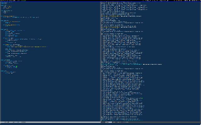
I write most of my code in Emacs, and my preferred setup is to have the window split horizontally with two buffers side-by-side:

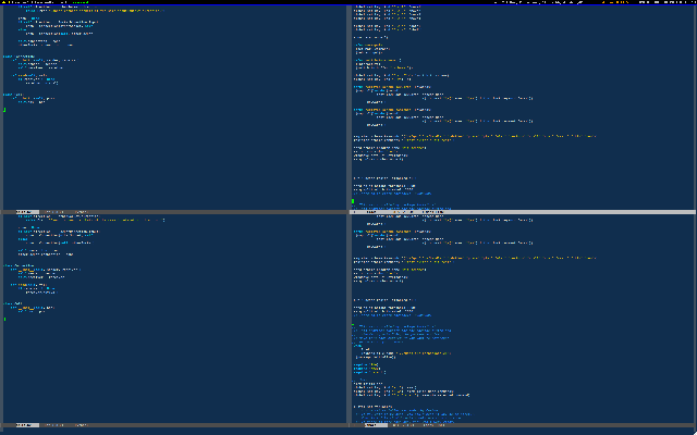
I find it frustrating when something automatically creates new splits and alters my layout instead of reusing the existing ones. This has been happening especially frequently since I got a high resolution screen, the Dell U3011. Emacs will keep splitting until the window is partitioned into a 2×2 grid whenever I run a command that outputs to its own buffer:

Personally, I find this behavior distracting and a waste of screen estate. To fix it, I added the following lines to my .emacs file:

(setq split-height-threshold 1200)
(setq split-width-threshold 2000)

Those values are somewhat arbitrary, but as a rule of thumb the higher the values the less likely Emacs is to create new splits. For full documentation, see the Emacs manual.

Based on my previous work on counting collocations, I created the website Semantic Link. Semantic Link allows you to search for words that are semantically related. Give it a try and see what word relations you discover!

How does it work?

Some words in the English language occur frequently together. One example is “Turing” and “Bletchley”, the former referring to the famous British computer scientist and the latter to Bletchley Park where he worked. We call such words semantically related, meaning that their co-occurrence is not due to chance but rather due to some non-trivial relationship. Such relationships include, for example, similar syntactic roles or similar meanings.

Semantic Link analyzes the text of the English Wikipedia and attempts to find all pairs of words which are semantically related. For that purpose it uses a statistical measure called mutual information, or MI for short. The higher the MI for a given pair of words, the higher the chance that they are related.

Semantic Link displays the top 100 related words for each query. The search is currently limited to words that have at least 1,000 occurrences in Wikipedia, but if there is enough interest I will gladly expand the database.

The tools used to generate the dataset for Semantic Link are licensed under GPL and are available for download at http://mpacula.com/autocorpus/.

My previous post, Counting Collocations: GHC and G++ benchmarked, created a bit of a controversy in the Haskell subreddit. The most common complaint was that the C++ and Haskell programs used different data structures which made the comparison unfair. Many people offered advice on how the Haskell code could have been improved in this regard. The top suggestions were:

  1. replace String with Text or ByteString
  2. replace Data.HashTable with Data.HashMap from the unordered-containers package

The first item was suggested because String operations are known to be notoriously slow, and any text processing application should use Text or ByteString instead. These alternatives are also closer to the array-of-bytes string representation in C++ and would provide a more fair comparison. Likewise, Data.HashTable is not a top performer and faster implementations exist. While I think these are very valid suggestions, let me digress for a moment and explain why I chose String and Data.HashTable in the first place.

My goal in the original article was not to come up with the fastest possible program in neither Haskell or C++, but rather to implement the same algorithm in a straightforward way using standard library types and functions and see how well the respective compilers could optimize it. None of my original implementations were written with performance in mind, nor did I manually tune them. I used String in Haskell simply because that’s what string literals evaluate to. Likewise, I used Data.HashTable because it comes with GHC.

That said, to many Haskell developers the notion of standard types and functions extends to packages included in the Haskell Platform and/or easily accessible through cabal. Since this seems to be the prevailing view, it would be dishonest not to report results for a Haskell collocation counter that uses faster data structures. The rest of this article describes the new implementation and presents the new benchmark numbers.

Improved Collocation Counter

The improved Haskell implementation was contributed by Bas van Dijk. You can view the source here. Compared to the original version, the notable changes are:

  1. Data.Text replaces most uses of String
  2. Data.HashMap.Strict replaces Data.HashTable
  3. a two-level hash map replaces the original
  4. a faster version of nub is used with performance instead of the default nub‘s
  5. sentences are stored as words which avoids redundant splitting inside sentenceCounts

The first two optimizations merely swapped data structures for faster implementations. The last three changed the overall algorithm and I had modify the C++ code accordingly in order to maintain a fair comparison. You can view the updated C++ code here.

Benchmark results follow.

Results

The hardware and software setup was the same as in the earlier benchmark, i.e. a 2.4GHz quad-core Q6600 Linux box with 6GB of memory running 64-bit Ubuntu 11.10. The benchmarks were compiled with -O2 optimizations using G++ 4.6.1 and GHC 7.0.3. Unless noted otherwise, all presented data points have been averaged over 30 runs. For individual run results, see data/collocations-{cpp,hs}-times.csv in the git repository.

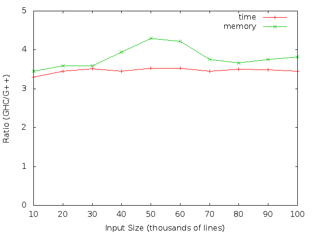
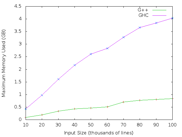
Figures 1 and 2 show the time and maximum memory used by the C++ and Haskell implementations as a function of input size in thousands of lines. Figure 3 shows the ratio of time and memory used by Haskell to the time and memory used by C++. On average Haskell was 3.47x slower and used 3.81x more memory than C++ on the same input. These relationships held regardless of input size, with a small deviation in the ratio of used memory between and .

Figure 1: Time taken by the C++ (G++) and Haskell (GHC) implementations as a function of input size. On average Haskell was 3.47x slower than C++ on the same input.

Figure 2: Maximum memory used by the C++ (G++) and Haskell (GHC) implementations as a function of input size. On average Haskell used 3.81x more memory than C++ on the same input.

Figure 3: Time and maximum memory used by the Haskell implementation relative to time and memory used by the C++ implementation. On average Haskell was 3.47x slower and used 3.81x more memory than C++ on the same input.

Tables 1 and 2 show the costliest calls (cumulative time) for the C++ and Haskell binaries for an input of 20 thousand lines. Please take these results with a grain of salt as they show only one run with compiler optimizations turned off. Due to space constraints, only the top functions are shown. For full information, the curious reader is welcome to look at the gprof and GHC profiler outputs.

function cumulative time (%)
main

99.5
documentCounts

98.5
std::sort

42.1
paragraphCounts

42.0
sentenceCounts

13.5
words

4.0
nub

1.3

Table 1: Costliest calls (cumulative time) of the C++ collocation counter. For function details, see Colocations.cpp.

function cumulative time (%)
main

73.5
serialize

31.6
countTable

19.1
counts

7.4
pairs

5.6
sentenceCounts

5.1
fastNub

4.2
convert

0.9

Table 2: Costliest calls (cumulative time) of the Haskell collocation counter. For function details, see Colocations.hs.

Conclusions

Bas van Dijk’s improvements to the Haskell collocation counter made its performance closer to the performance of the same algorithm implemented in C++. On average Haskell was 3.47x slower and used 3.81x more memory than C++ on the same input, which is a significant improvement from the previous 5.91x and 4.95x. Since I considered the old numbers to be pretty pretty good by themselves, I think this is a great result. A 3.47x slowdown is a small price to pay for the simplicity and convenience of Haskell as a language, and is a testament to how well GHC can optimize Haskell programs.

Lies, damned lies, and benchmarks.

Note: the GitHub code has since been updated. You can see the implementation this post is referring to by viewing the “1.0” tag.

I have been investigating various methods of statistically inferring synonyms from natural language corpora. As a part of my investigation, I implemented a method based on collocation counting, where two words are considered likely to be synonyms if they tend to occur close to each other in the training corpus. Since counting collocations is a CPU and memory intensive problem, I implemented my solution in two languages which I knew had excellent compilers: C++ (G++) and Haskell (GHC). I then benchmarked the compiled binaries in terms of speed and memory use. Both of my implementations were algorithmically equivalent and emphasized simplicity and ease of development over performance. As such I believe they provide a measure of relative performance that users of C++ and Haskell can expect from similar programs without manual optimizations. In this article I present the results of my evaluation.

Background

When using collocations for synonym inference, it is assumed that two words and are more likely to have a related meaning if they tend to occur close together. This is captured by a metric called mutual information [1]:

The individual probabilities can be estimated from data. For simplicity, assume we are using maximum likelihood estimates based on some language corpus . then becomes the frequency of in , and the frequency of occurring in close proximity to . What constitutes proximity depends on the implementation. One popular approach is to use absolute word distance: and are considered in each other’s proximity if they are separated by at most words, being a parameter of the model. Another approach is to use sentence distance, defined analogically. In my implementation I use sentence distance with . I furthermore ignore words in the current sentence and only consider words in adjacent sentences as neighbors (e.g. if the words “a” and “b” are present in the current sentence but “b” is not in any adjacent sentence, “a” and “b” will not be considered neighbors).

An adept reader will notice that a key element of estimating mutual information is counting proximal word pairs in a language corpus. Conceptually, this is a simple problem: for each word in the corpus and for each word near produce the count and then tally up the counts. In practice, however, the large size of the language corpus makes this a lengthy and memory-consuming operation. It is easy to see why: assuming a dictionary of possible words, in the worst case we will produce counts for each possible pair – a total of count pairs. Even for a modest dictionary of size 10000, this amounts to 10 billion count pairs.

When implementing a collocation counter, it is therefore imperative to choose a programming language and a compiler that produce efficient code. While C/C++ (G++) are natural candidates, according to the The Computer Language Benchmarks Game Haskell (GHC) is a worthy contender, being on average only 2.5x slower than G++ on a wide set of benchmarks. This seems like a small price to pay for the niceties of the language.

However, the data from The Computer Language Benchmarks Game can be a bit misleading as it only compares the fastest implementations in each language. As such, it only provides kind of an upper bound on the performance that a user can expect from a compiler. While tremendously useful in many application, it does not reflect the performance of a typical, idiomatic program in each language. This “typical performance” is what I attempted to measure in this article for the particular use case of counting collocations.

Implementation

The source code of my C++ and Haskell collocation counters is available on GitHub. Both implementations follow the same general algorithm:

get_counts(sentence, context):
  count_list=[]
  for w in words(sentence):
    for v in unique_words(context):
      count_list.append((w,v,1))
  return count_list
 
count_colocations(input):
  counts = new HashMap
  counts[w1 <- V, w2 <- V] = 0
  for paragraph in input:
    for sentence in paragraph:
      context = get_adjacent_sentences(sentence, paragraph)
      for (w,v,c) in get_counts(sentence, context):
        counts[w,v] += c
   return sort_by_words(to_association_list(counts))

The only thing of note is that get_counts returns a list of counts instead of directly accumulating the counts in the hash map, which is arguably non-idiomatic in the imperative C++. I made this particular choice to keep get_counts pure in Haskell, which would otherwise have to use Data.HashTable in the IO monad.

Both C++ and Haskell implementations read all their input into memory first (albeit Haskell does this lazily) from stdin and print the counts to stdout, one per line.

Results

I evaluated both implementations on an excerpt of plaintext Wikipedia articles generated with AutoCorpus. The full dataset is available in the GitHub repository as data/input.txt. The test system was a 2.4GHz quad-core Q6600 Linux box with 6GB of memory running 64-bit Ubuntu 11.10. The benchmarks were compiled with -O2 optimizations using G++ 4.6.1 and GHC 7.0.3. Unless noted otherwise, all presented data points have been averaged over 30 runs. For individual run results, see data/collocations-{cpp,hs}-times.csv in the git repository.

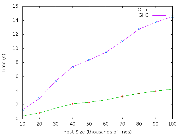
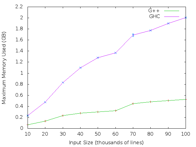
Figures 1 and 2 show the time and maximum memory used by the C++ and Haskell implementations as a function of input size in thousands of lines. Standard deviation was minimal and, while shown, cannot be discerned in the plots. Since both implementations ran essentially the same algorithm, the overall shape of the time and memory curves is identical as expected. On average, Haskell was 5.91x slower than C++ on the same input and used 4.95x more memory. This relationship held to within 0.9x regardless of the size of the input.
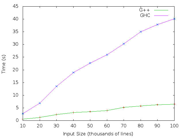
Figure 1: Time taken by the C++ (G++) and Haskell (GHC) implementations as a function of input size. On average Haskell was 5.91x slower than C++ for the same input.

Figure 2: Maximum memory used by the C++ (G++) and Haskell (GHC) implementations as a function of input size. On average Haskell used 4.95x more memory than C++ for the same input.

Tables 1 and 2 show the costliest calls (cumulative time) for the C++ and Haskell binaries for an input of 20 thousand lines. Please take these results with a grain of salt as they show only one run with compiler optimizations turned off. Due to space constraints, only the top functions are shown. For full information, the curious reader is welcome to look at the gprof and GHC profiler outputs. The visualized C++ call graph is also available here.

function cumulative time (%)
main

100
documentCounts

98.7
paragraphCounts

54.9
sentenceCounts

38.7
std::sort

31.7
words

29.1

Table 1: Costliest calls (cumulative time) of the C++ collocation counter. For function details, see Colocations.cpp.

function cumulative time (%)
main

100
documentCounts

48.7
paragraphCounts

28.1
sentenceCounts

27.9
sentenceToSet

22.5
aggregateCounts

19.5

Table 2: Costliest calls (cumulative time) of the Haskell collocation counter. For function details, see Colocations.hs.

The time profiles of the two programs are very similar. The difference between the times spent in documentCounts is due to the C++ implementation performing sorting inside that method, while the Haskell implementation does it directly in main. Curiously, the profiler indicates that over 70% of the individual time of the Haskell program was spent in the GC module (see GHC profiler output), suggesting that garbage collection might be the culprit of Haskell’s slower performance.

Conclusions

A naive collocation counting algorithm in Haskell (GHC) was 5.91x slower and used 4.95x more memory than the same algorithm implemented in C++ (G++). The interpretation of these results is up to the reader. Personally, I think the slowdown is a reasonable trade-off for the productivity benefits of Haskell as a language, and I suspect it is still significantly faster than an equivalent algorithm implemented in a popular scripting language like Python, Perl or Ruby (although I have no data to back up that claim ;-)).

References

  1. M. Baroni, S. Bisi. Using cooccurrence statistics and the web to discover synonyms in a technical language. Proc. of the Fourth International Conference on Language Resources and Evaluation (LREC 2004). 2004.

I just released AutoCorpus 1.0.1. AutoCorpus is a set of utilities that enable automatic extraction of language corpora and language models from publicly available datasets such as Wikipedia. It consists of fast native binaries which can process tens of gigabytes of text in little time.

AutoCorpus utilities follow the Unix design philosophy and integrate easily into custom data processing pipelines.

Homepage: http://mpacula.com/autocorpus
GitHub: https://github.com/mpacula/AutoCorpus

M.Eng. thesis It’s finished! After almost 2 years of research and months of writing, I finally submitted my Master of Engineering thesis to the department. In this post, I would like to thank the many people who have made my past 5 years at MIT such an extraordinary experience: Joel Moses for being a great academic advisor, Una-May O’Reilly for her endless enthusiasm and invaluable advice as my thesis supervisor, the many amazing professors in my classes, and finally my friends and family. Thank you all!

My finished thesis, titled “Evolutionary Algorithms for Compiler-Enabled Program Autotuning”, is available here:
http://mpacula.com/publications/mpacula-meng-2011.pdf.

Abstract

PetaBricks is an implicitly parallel programming language which, through the process of autotuning, can automatically optimize programs for fast QoS-aware execution on any hardware. In this thesis we develop and evaluate two PetaBricks autotuners: INCREA and SiblingRivalry. INCREA, based on a novel bottom-up evolutionary algorithm, optimizes programs offline at compile time. SiblingRivalry improves on INCREA by optimizing online during a program’s execution, dynamically adapting to changes in hardware and the operating system. Continuous adaptation is achieved through racing, where half of available resources are devoted to always-on learning. We evaluate INCREA and SiblingRivalry on a large number of real-world benchmarks, and show that our autotuners can significantly speed up PetaBricks programs with respect to many non-tuned and mis-tuned baselines. Our results indicate the need for a continuous learning loop that can optimize efficiently by exploiting online knowledge of a program’s performance. The results leave open the question of how to solve the online optimization problem on all cores, i.e. without racing.

I recently migrated my data from one server to another, and decided to convert some old Subversion repositories to Git. Turns out such conversions require more typing than I would like, so I made a simple bash script to automate the process (see below). The script, svn-to-git, takes two parameters:

  1. the source Subversion repository (has to be local)
  2. the destination Git repository (will be created automatically)

Note that the import is rather simplistic and you might want to expand the call to git svn on line 30. The defaults should be enough for the common use cases, however.

Download the script here.

#!/bin/bash
echo "This script converts an SVN repository into a Git repository."
printf "%-15s $1\n" "[source]:" 
printf "%-15s $2\n" "[destination]:"
 
script_name=`basename "$0"`
src="$1"
dest="$2"
 
if [ ! -e "$src/db" ]
then
    echo "ERROR: '$1' does not appear to be a Subversion repository." >&2
    exit 1
fi
 
if [ -e "$dest" ]
then
    echo "ERROR: '$dest' already exists." >&2
    exit 1
fi
 
mkdir -p "$dest"
cdir=`pwd`
cd "$src"
abs_src=`pwd`
cd "$cdir"
 
tmp_dir="/tmp/$script_name-$$"
echo "Cloning repository into $tmp_dir..."
git svn clone --local "file://$abs_src" "$tmp_dir"
 
echo "$tmp_dir -> $dest"
git clone "$tmp_dir" "$dest"
 
echo "Cleaning up..."
rm -rf "$tmp_dir"
 
echo -e "\nDone! You can access your new Git repository at '$dest'."
echo "Good day."