Testing any kind of software is difficult. The programmer is faced with a multitude of choices and trade-offs: what components to test and in what scenarios, how much time to spend writing test cases vs. developing new features, and so on. No matter how hard, many acknowledge that testing is paramount to producing a quality product. So important, in fact, that companies like Microsoft make software testing a full-time position.
And if testing most software is hard, testing statistical software is even harder. For most of my programming career I hardly had to deal with statistics and “big data” problems. As a result, when I embarked upon my first significant statistical project a year ago, it proved to be a major source of frustration. In this post I hope to share my experiences with testing statistical code. I will start by describing my initial sources of difficulty stemming from the differences between statistical and non-statistical programs. I will then present a number of testing guidelines which I have found to be particularly effective, and which avoid some of the pitfalls I would initially get myself into.
The initial discussion and guidelines are primarily about probabilistic software, which is just a subset of the possible statistical programs you could write. However, later sections deal with statistical software in more generality.
How Many Outcomes?!
Testing non-statistical software components often involves executing some action which can result in some fixed number of outcomes, and then verifying that the actual outcome is what we expected. For example, one might write the following code in Java:
Set<String> hat = new HashSet<String>(); hat.add("rabbit"); Assert.assertTrue(hat.contains("rabbit")); |
In the above case, there are two possible outcomes of an “insert” operation: either the set contains the added element, or not. Having inserted an element into the set, we check whether the outcome is what we want it to be. Of course, in real programs tests are more complicated and often involve a significantly larger number of possible outcomes. However, the outcomes still usually form a set of a manageable size.
Statistical code differs in two significant ways:
- there are several orders of magnitude more possible outcomes of an operation
- it is often not obvious which outcomes are correct
I will try to illustrate the impact of the two points above on an example. Consider a Maximum Likelihood Estimator (MLE) – arguably one of the simplest statistical tools. An MLE counts the occurences of an element in a sequence of observations , and uses that to estimate the probability of that element. For example, if you observe three dogs and two cats, then an MLE would estimate the probability of each as 0.6 and 0.4, respectively. Notice how the outcome of an MLE is a number – a number that we cannot conveniently restrict to a small set of possible values. Not even in the range 0-1, since we cannot make correctness assumptions about the very thing we are testing. It can be said that despite the large number of possible outcomes, it is straightforward to say which are correct. That is often not the case, however, as the dataset might be too large or the model too complex to manually estimate probabilities. And even in cases when such manual estimation is possible, it is all to easy to make mistakes.
To make matters worse, the naive MLE is an oversimplified example. Consider only a slightly more sophisticated estimator, called an Absolute Discounting Estimator (ADE). An ADE subtracts a (small) probability mass from seen events, and distributes it across unseen events. This process of transferring probability mass, so called “smoothing”, is of paramount importance in applications such as spam classification and statistical Natural Language Processing. Let’s first define an ADE mathematically: let be the sequence of observations, where each observation belongs to a set of possible events, and let be a constant which controls the amount of smoothing. An ADE is then defined as:
While only slightly more complicated than an MLE, testing the ADE on large datasets can be a nightmare if you simply compare hard-coded estimates. You have to test that the ADE behaves correctly for different values of , and possibly on different datasets. It would be a Herculean task to manually compute all those probabilities, and then test the ADE against these estimates. That’s what I used to do as a beginner, and calling my experiences frustrating would be an understatement.
Obey Probability, It’s The Law!
Luckily, when it comes to probability, there are a few simple guidelines that make testing much easier. They might sound obvious to many, but the obvious sometimes needs pointing out, especially if our mindset is from another, non-statistical domain.
A great thing about probability is its extensive mathematical foundation, and the fact that it obeys several rather simple laws. Instead of testing the returned values directly, test that your components behave properly with respect to the laws of probability. No matter how complicated your model, or how large the test dataset, these laws should always hold. Always. Some of the laws I have found particularly useful are outlined below.
Stay positive
Make sure that every probability produced by your code is non-negative. While this may sound trivial, in many cases it is not. Consider the ADE formula I showed earlier – it has a flaw that might not be immediately obvious. Namely, if , we will get negative probabilities for infrequent elements! This problem might be extremely hard to track down in production, since the wrong answer produced by an ADE will usually be propagated through a long chain of other mathematical operations.
Be normal(ized)
If your code defines a discrete probability distribution, as in the case of a classifier, make sure that the probabilities of all events add up to one. Since this test requires your code to produce probabilities for all possible arguments, it has a good chance of detecting miscalculations for any single one.
Know your maginals
I have found marginalization to be extremely useful for testing classifiers, and it applies to other kinds of programs, too. It relies on the formula:
In many cases, you know the value of (for example, it might be your prior), and you know how to compute with the component you are testing. And even if you do not know , you can often compute it using conditional probabilities:
.
Similarly to normalization, marginal probabilities require you to compute probabilities for all possible values of an argument, and are good at catching any single miscalculation. They also have another advantage: you only have to sum over the possible values for one argument, which is computationally cheaper than summing over possible values for all arguments, as would be required by normalization.
Of course, the above list of probability laws is by no means exhaustive, and it is always a good idea to open a probability textbook and search for formulas that apply directly to your problem. For example, there is a large body of theory behind Markov Chains, and if Markov Chains is what you are testing, the relevant formulas will probably be better at testing your code than the general laws outlined above. No matter what laws you end up using in your code, however, the message is the same: try to avoid testing exact values if possible, as they are too parameter-dependent and too hard to correctly calculate manually – and use probability laws instead.
All Your Baseline Are Belong To Us
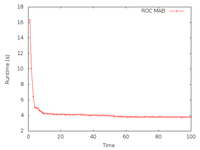
A good way to test any statistical software is to compare its performance against some reasonable baseline. For example, suppose you are developing a very sophisticated reinforcement learning system, and initial tests show great performance. The problem is that “great” is relative, and you never truly know how good your method is until you compare it to something else. Last week I was working with my CSAIL collegues on a paper for a large Machine Learning conference. We devised a clever method to apply Multi-armed Bandit techniques to online multi-objective tuning of computer programs. We gathered a lot of data, did statistical analysis and then plotted the average performance of a benchmark program as a function of time (lower is better):

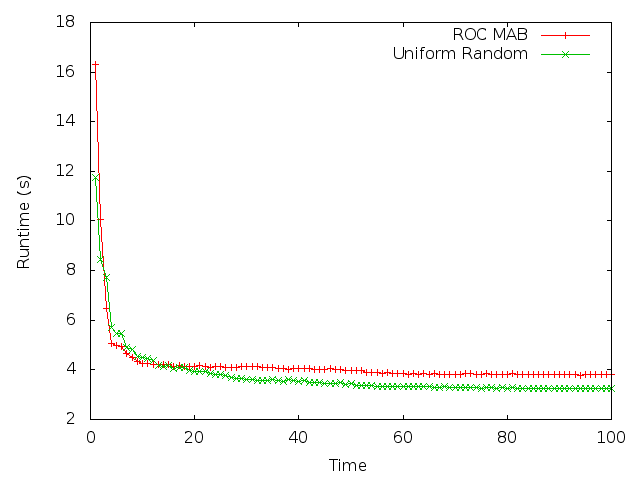
We were excited since our approach seemed to converge very fast, and reduced the runtime of the benchmark by a significant amount. However, we then compared the performance of our method to a naive, “uniform random” baseline. Here is what we saw:

Uniform random clearly outperformed our method, regardless of how good the results initially looked. This allowed us to discover a major problem with our methodology – we did not correctly optimize hyperparameters. It also emphasized how important and useful it is to test your code against a baseline. Not only will it show how well your code performs, but also whether it performs worse than you expect it to. If it does perform worse, it might indicate a serious bug, as it did in our case.
You might argue that baseline testing is not really useful as a unit test, since it involves looking at plots and making inferences about behavior, but that is not necessarily true. There are many ways you can programmatically compare the performance of one method against another, such as Student’s t-test. It was in fact a t-test analysis of our benchmark data that allowed us to conclude that our buggy program was no better than a naive approach.
It’s All Magic!
My final point is not so much about writing unit tests, but about designing for testability. A few years ago, before I took any formal courses in probability and statistics, I would often use “magic”, ad-hoc scores for various things to indicate, for example the “likelihood” that candidate is better than candidate . While in many cases using such ad-hoc scores can seem straightforward and their use tempting, they are a nightmare to test. This is due to the fact that there is usually no sound theory to support them, and if you want to evaluate their performance and/or test them you cannot rely on any laws or tried analysis tools. Because of this, try to resist the temptation to use magic scores and other such metrics, no matter how straightforward to implement they are. More often than not, as I learned all too well, they will only lead to problems later on. Whenever possible, try to re-formulate your problem in terms of probabilities and other well-founded metrics. I wish somebody had said this to a younger me – how many hours of frustration it would have saved!
Go Forth and Estimate
That’s it, folks. In this article I tried to describe why, in my opinion, statistical software is much harder to test compared to “ordinary”, non-statistical programs. I argued that it was due to the sheer number of possible outcomes that statistical components can produce, and it is not always immediately obvious which of those outcomes are the correct ones. I gave a few guidelines that I personally found very useful when testing various kinds of statistical programs – both probabilistic and non-probabilistic. Finally, I made a case why magic, ad-hoc scores should not be used in place of probability whenever possible.
I hope you found my entry useful – there’s surprisingly little about testing statistical code on the Internet. As always, please let me know your thoughts and comments. Now, go back to your statistical programs and estimate (hopefully correctly)!
Thanks to Daniel Firestone for reading drafts of this article.
45 responses
Do you want to comment?
Comments RSS and TrackBack Identifier URI ?
Trackbacks